How to Use Conditional Formatting Based on Another Cell?

In this tutorial we are learn about how to conditional formatting based on another cell? In this tutorial we will learn how to create different formatting rules, how to edit and copy our formatting rules in ms excel, and also how to do conditional formatting based on another cell. It is a really powerful feature when it comes to applying different formats to data that meets certain condition. It can help you highlight the most important information in your spreadsheets and identify variances of cells' values with a quick glance.
How to create conditional formatting rules?
1.      First select the range of cell which we want to create conditional formatting.
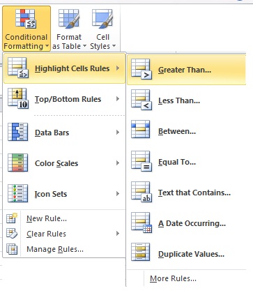
2.      Then we go to conditional formatting command and press the option we will see the drop
         down list.
3.       And select the Highlight cell rules, and select Greater than option.

4. when we select the Greater Than option we see a Greater than option as given in below image.

In this image we see, First when we want to format cell greater than 1000,so we will enter the value of 1000. He highlights the number which is greater than 1000. Same process do in all option.

Preset conditional formatting
Microsoft excel has several presets we can use to quickly apply conditional formatting to your cells. They are grouped into three categories:

1.      Data Bars
2.      Color Scales
3.      Icon set

Data Bars:- First we discuss about Data bars, Data bars are horizontal bars added to each cell, much like a bar graph.

Note:-  Its not work when we select the alphabetical cell. Its work when we select Numerical cell.

Color Scales:- Now we discuss about Color Scales, Color scales change the color of each cell based on its value. Each color scale uses a two- or three-color gradient. For example, in the  -Yellow-Red- Green  color scale, the highest values are yellow, the average values are red and the lowest values are green.

Icon set:-  Now we discuss about Icon Sets, Icon sets the change the color of each based
on its value. Each directional sign shows icons in data cells by applying desired Condition.

For Example, Red sign is low number yellow sign shows medium number and green sign shows highest number.

In above image shows that Red color show Lowest Number, yellow color shows Medium Number and Green color shows Highest Number.We also choose shapes, indicators and Ratings to show the Numbers.

For More icon set ruler, we will go to conditional formatting select Icon sets and go to more rules and press it. Now we see New formatting Rule box as image given as below.

In this image we will go to Select a Rule Type and select Format all cells based on their values the go to Edit the Rule Description and We set format all cells based on their Values as we want.
If you have found any mistake or have any doubt related to above how to conditional formatting based on another cell? tutorial then comment below. If you like the tutorial the follow on twitter and also like us on facebook.